To start using our app, you are required to create an account and provide minimal information about yourself. Once you have an account, you will see “Profile” tab (a red box #1 in Figure 1), which allow you to choose your preferred spatial unit (ft vs m) and optionally turn on color blind settings. Now you are ready to start using our app, if you are using the public data available through our online database. Clicking “Explore” button located on the top right corner (a red box #2 in Figure 1) will direct you to the GIS layer page visualizing the map of California.
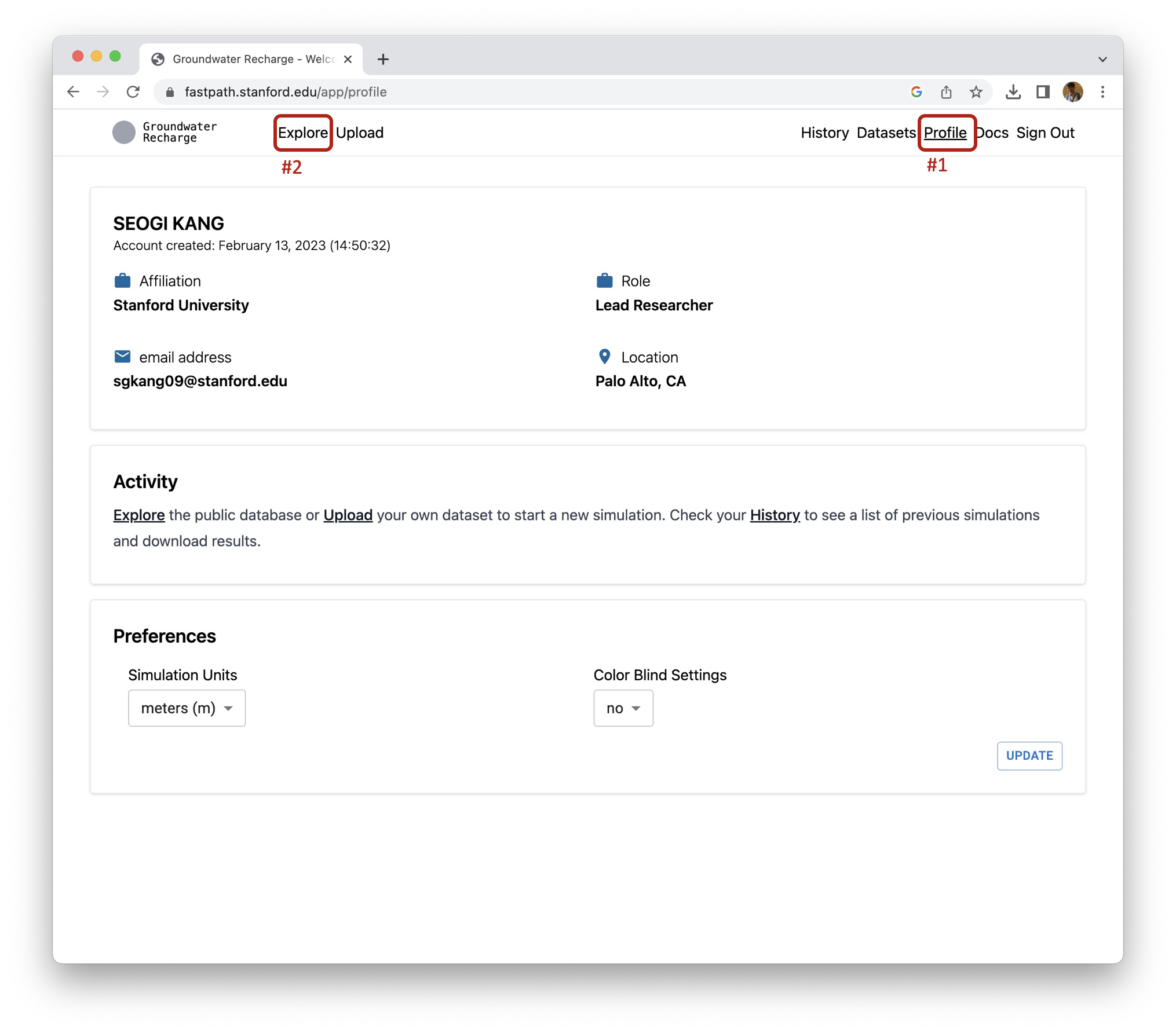
Figure 1:An example webpage for a user account.
Using user’s data
This section addresses the case where you want to use your own EM and sediment-type data and/or mix your data with the public data in our database. If you want to upload your own EM and/or sediment type data, you need to click “Upload” button located right next to “Explore” button (a redbox #2 in Figure 1). Then you would see the webpage shown in Figure 2. You can upload EM data and/or sediment type data, which will then be stored for you.
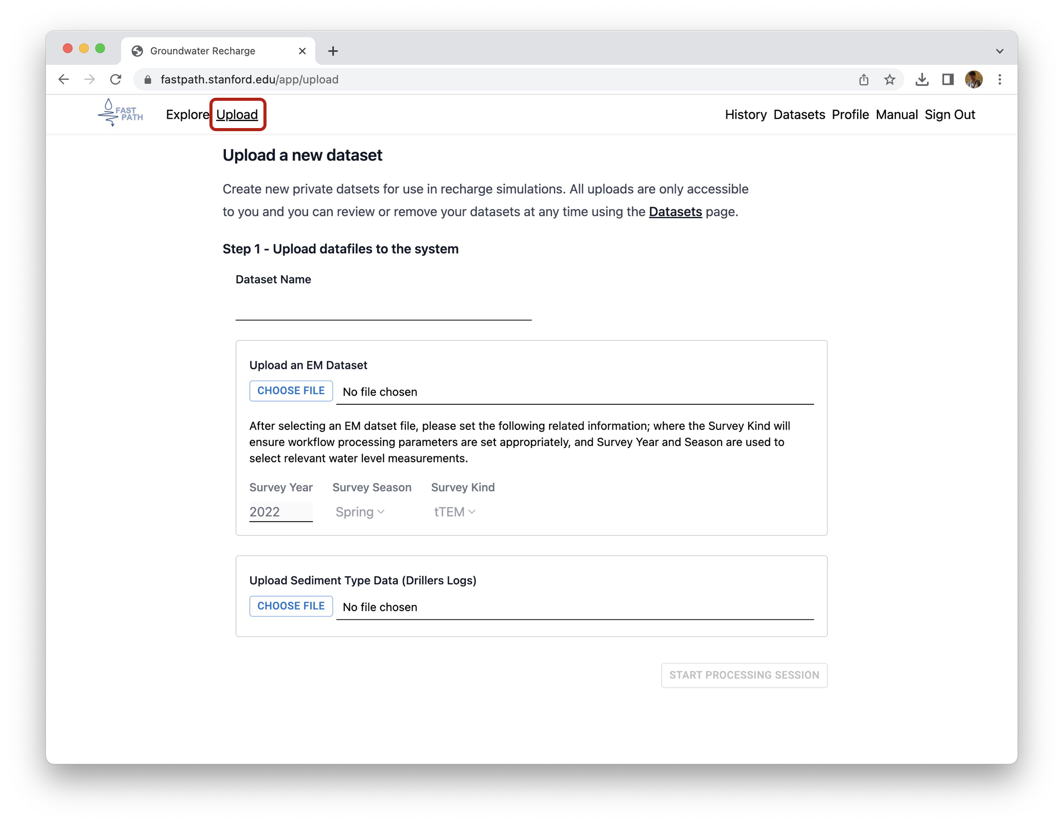
Figure 2:Webpage allowing user to upload user’s own data.
EM data
When uploading the EM resistivity data – a 1D vertical resistivity profile defined at each location –, you required to fill in Survey Year, Survey Season, and Survey Kind. The first two items are needed to select the water level measurements acquired corresponding year and season. The last item, survey kind (either AEM or tTEM) is needed for determining parameters used in the web-application. Input data should be in MOD_inv.xyz format exported from the Aarhus workbench. When the EM data inverted using the workbench and exported, there are three files:
Filename_MOD_inv.xyz: includes the resistivity data.Filename_MOD_dat.xyz: includes the observed voltage data.Filename_MOD_syn.xyz: includes the predicted voltage data from the EM inversion.
If you did not use the workbench to invert the EM data, then it is your responsibility to convert the output to the workbench’s MOD_inv.xyz format. Example resistivity data exported from the workbench are available at the below link:
Sediment type data
For the sediment data, you need to compile a csv (comma-separated values) file. This includes the location of the well data in a specified UTM (Universal Transverse Mercator) coordinate system: NAD83 California Albers [in meters]: EPSG 3310, and sediment type at each vertical interval in the log. User’s csv file should include five columns as shown in :
WellID: ID for a well.SEDIMENT_TYPE:coarse,fine, orunknown(all lower case); any other types will be considered asunknown.top_meter: top of the vertical interval [m].bottom_meter: bottom of the vertical interval [m].UTMX: X coordinate; NAD83 California Albers [m]UTMY: Y coordinate; NAD83 California Albers [m]
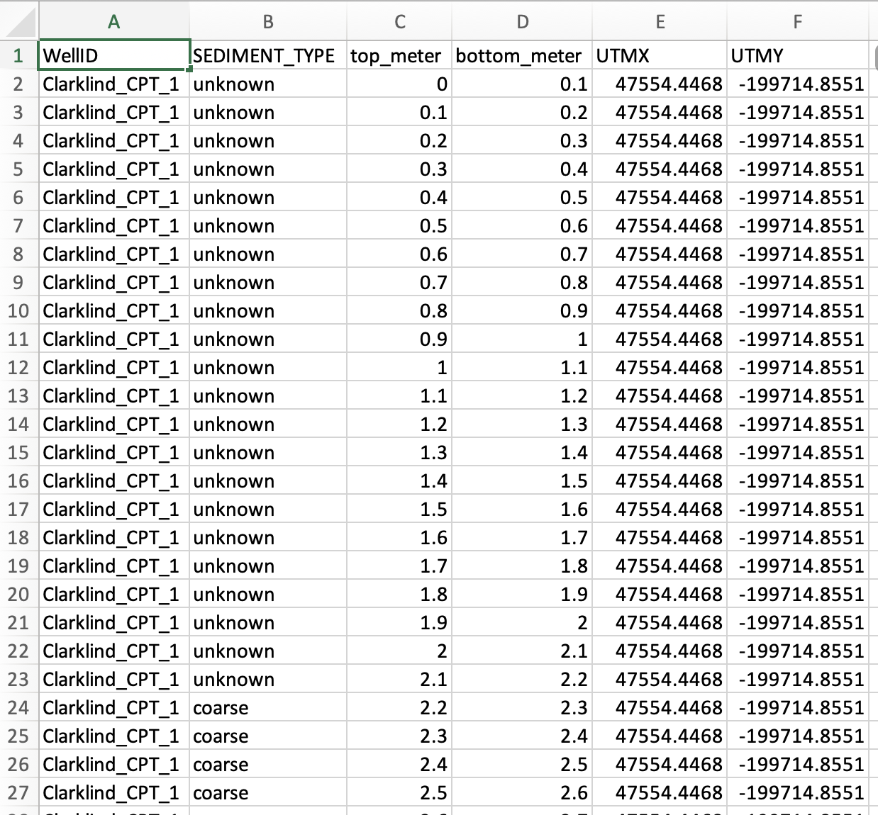
Figure 3:Example csv file for the sediment type data.
Example sediment type data are available at the below link:
After the upload
Once you finish uploading the data (by clicking “START PROCESSING SESSION”), you will see a webpage similar to Figure 4.
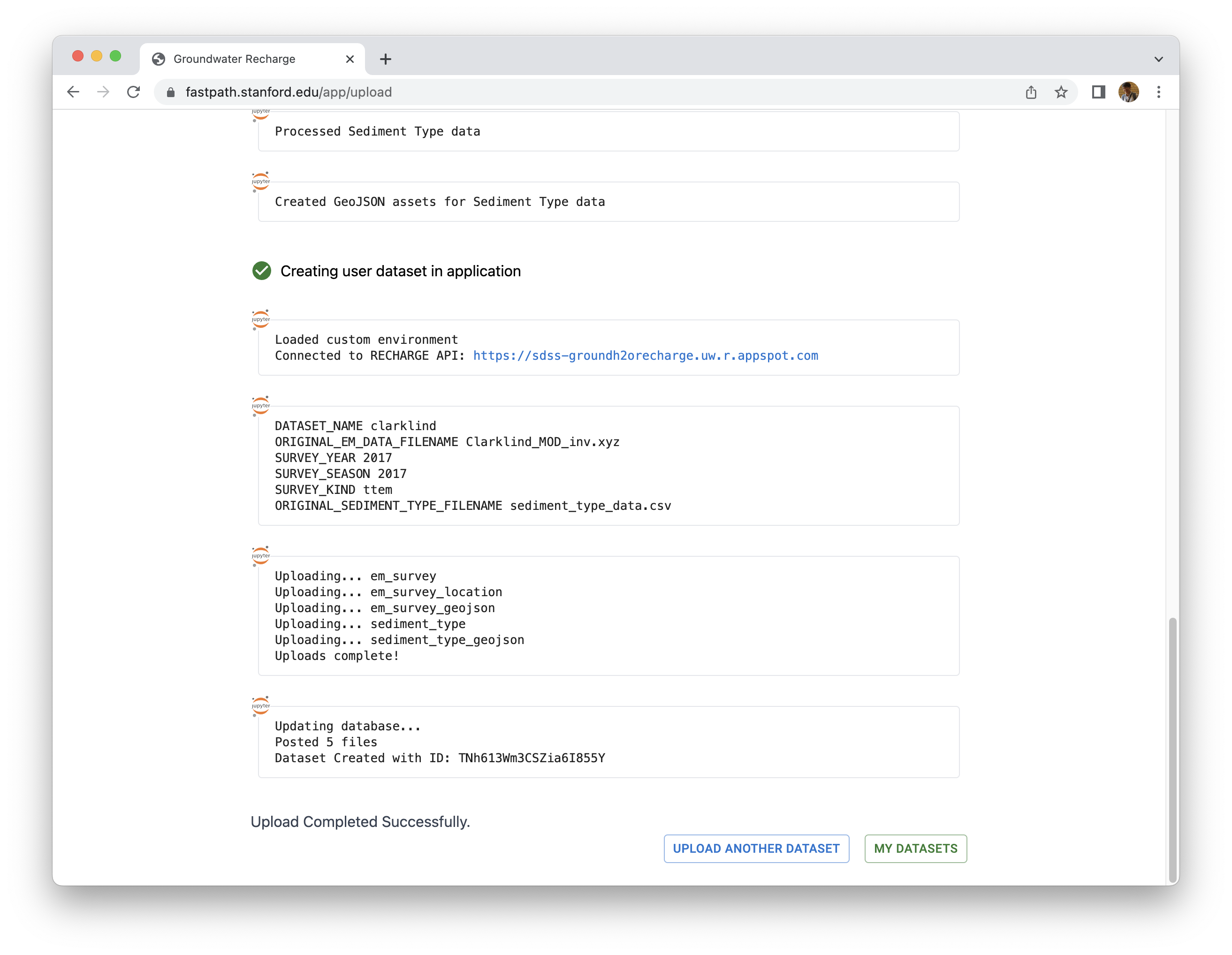
Figure 4:An example webpage after uploading the user’s data.
Then if you click “MY DATASETS” button, you will see a webpage similar to Figure 5. These data will be accessible on the GIS layer that I am going to explain in the next section: GIS layer.
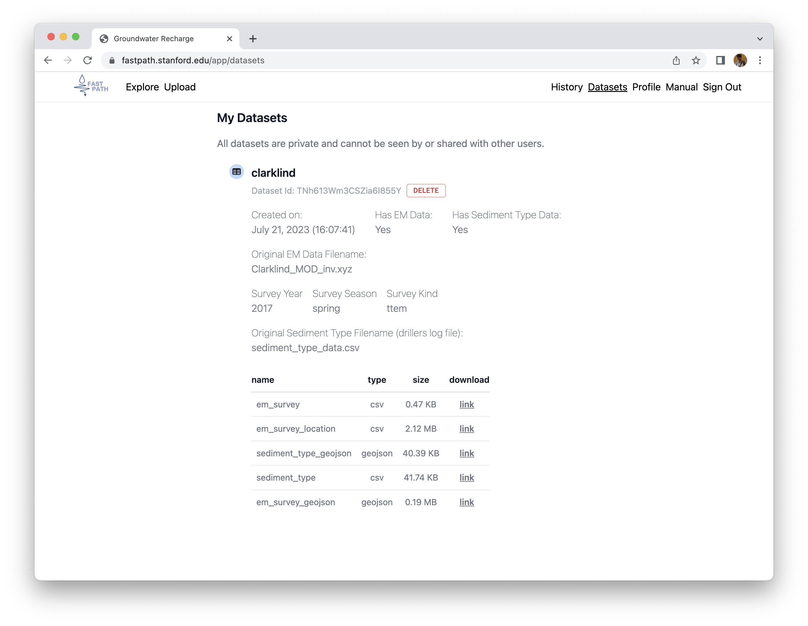
Figure 5:An example webpage showing the uploaded user’s data into the fastpath app.